Fast, Broadcasted Mueller Polarimetry

written by Jaren N. Ashcraft

katsu was built in part to understand the spatially-varying polarized response of optics. Manufacturing errors can leave phase and amplitude aberrations in an optical beam, and understanding these sources of error is critical to understanding our system.

To spatially resolve this data, we need to be able to do full polarimetry on an array of pixels - so a naive implementation of the algorithm will take a very long time to run. Here, we show off the numpy optimizations done to speed up the polarimetric data reduction for Full Mueller Polarimetry.

Readers should first be familiar with the Full Mueller Polarimetry demo

from katsu.polarimetry import (
    broadcast_kron,
    broadcast_outer
)

from katsu.mueller import (
    linear_polarizer,
    linear_retarder,
    linear_diattenuator
)

import numpy as np
from time import perf_counter

Polarimetric data reduction boils down to matrix multiplications and Kronecker products. Numpy is already configured to broadcast matrix multiplications, just stuff the matrix dimensions into the final two axes of the numpy array! But np.kron is a more general operation that operates on tensors of arbritrary dimension. A naive implementation of looping over the broadcasted dimensions would look like the following:

array_of_matrices = np.random.random([128,128,2,2])
array_out_naive = np.zeros([128, 128, 4, 4])

t1 = perf_counter()
for i in range(array_of_matrices.shape[0]):
    for j in range(array_of_matrices.shape[1]):

        array_out_naive[i,j] = np.kron(array_of_matrices[i,j], array_of_matrices[i,j])

runtime_naive = perf_counter() - t1
print(runtime_naive,'s to compute naive kronecker')

0.6168796999991173 s to compute naive kronecker

This is perfectly acceptable, but may scale unfavorably for large datasets that are highly sampled. In contrast, the implementation in katsu.katsu_math has configured the kronecker product using np.einsum, which batches the computation in the broadcast dimensions by assuming that we operate on a 2D matrix.

array_out = np.zeros([128, 128, 4, 4])

t1 = perf_counter()
array_out = broadcast_kron(array_of_matrices, array_of_matrices)
runtime_broadcast = perf_counter() - t1
print(runtime_broadcast,'s to compute broadcast kronecker')
print(runtime_naive / runtime_broadcast,'x relative speedup from naive implementation')

0.0041782000043895096 s to compute broadcast kronecker
147.64245353287046 x relative speedup from naive implementation

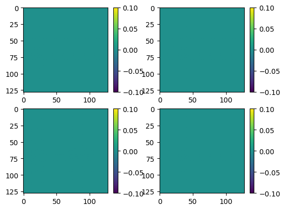
Just by virtue of a more specialized implementation, we can achieve significant runtime increases over the looped case! Furthermore, the results are functionally identical. Below we plot the difference of the elements of the matrix as a function of the first two array dimensions and observe that the results are entirely zero.

import matplotlib.pyplot as plt
difference = (array_out_naive - array_out)

def plot_square(x,n=2,vmin=None,vmax=None):
    k = 1
    plt.figure()
    for i in range(n):
        for j in range(n):
            plt.subplot(n,n,k)
            plt.imshow(x[..., i, j], vmin=vmin, vmax=vmax)
            plt.colorbar()
            k += 1
    plt.show()

plot_square(difference)

This is a no-compromise method of doing broadcasted kronecker products for Mueller matrices, and is our default for Mueller polarimetry in katsu, which we demonstrate below. We begin by constructing a simple Mueller Matrix. It is composed of a linear polarizer and retarder oriented at random angles.

M_simple = linear_retarder(np.random.random(),np.random.random()) @ linear_diattenuator(np.random.random(),np.random.random())
print('Mueller Matrix')
print(M_simple)

Mueller Matrix
[[ 0.54011332  0.45791451  0.04254481  0.        ]
 [ 0.37054239  0.43740045 -0.00369337 -0.16185025]
 [ 0.00411028 -0.02055424  0.27340817 -0.07119707]
 [ 0.27235492  0.31332204  0.08527031  0.22127383]]

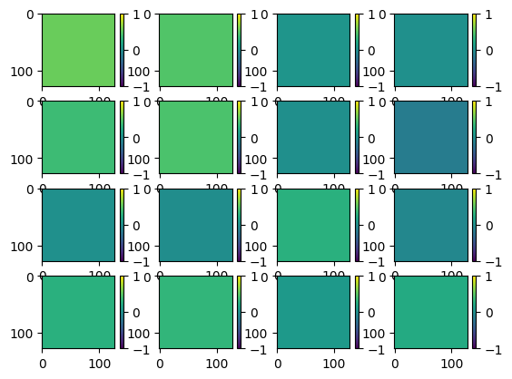
We now need to extend it to a spatial dimension, let’s maintain the size of the previous example and make the Mueller matrix array larger.

M_spatial = np.broadcast_to(M_simple,[128,128,*M_simple.shape])
plot_square(M_spatial, n=4, vmin=-1, vmax=1)

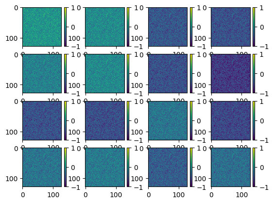
Now we create a noisy array and subtract it from each element of M_spatial to simulate a random polarization variation in a beam.

noisy_mask = np.random.random([128,128])
M_noisy = M_spatial - noisy_mask[..., np.newaxis, np.newaxis]
plot_square(M_noisy, n=4, vmin=-1, vmax=1)

Okay we’ve cooked up our Jones Matrix with spatial variation, but can we detect it? First we need to create our synthetic power measurement, and for that - we need a Mueller matrix model of our system. We begin by constructing the Mueller matrix for the polarization state generator Mg and the analyzer Ma.

In the below cell we are showing a little bit of how full_mueller_polarimetry works, so there’s a lot of shape manipulation of numpy arrays in order to broadcast the operations. This is just to make the code faster, so feel free to pay it no mind.

starting_angles={'psg_polarizer':0,
                'psg_waveplate':0,
                'psa_waveplate':0,
                'psa_polarizer':0}

nmeas = 26
thetas = np.linspace(0,2*np.pi,nmeas)

psg_qwp = linear_retarder(starting_angles['psg_waveplate']+thetas,np.pi/2, shape=[128, 128, nmeas])
psg_hpl = linear_polarizer(starting_angles['psg_polarizer'], shape=[128, 128, nmeas])

psa_qwp = linear_retarder(starting_angles['psa_waveplate']+thetas*5,np.pi/2, shape=[128,128, nmeas])
psa_hpl = linear_polarizer(starting_angles['psa_polarizer'], shape=[128, 128, nmeas])


Mg =  psg_qwp @ psg_hpl
Ma = psa_hpl @ psa_qwp

Now we compute the mueller matrix of the total system Msys

# reshape noisy array for matrix multiplication
M_noisy_broadcast = np.broadcast_to(M_noisy,[nmeas, *M_noisy.shape])
M_noisy_broadcast = np.moveaxis(M_noisy_broadcast,0,2)

# compute the system Mueller matrix
Msys = Ma @ M_noisy_broadcast @ Mg

Since the first optic is a polarizer, it truly doesn’t matter what polarization is incident on Msys, it all gets converted to linear polarization. Consequently, we can consider multiplying Msys by a Stokes vector equal to \(S = [1, 0, 0, 0]\) to retrieve the measured flux. This means that we measure the top-left element of the Mueller Matrix \(M_{sys,0,0}\) or, in numpy…

power_measured = Msys[...,0,0]

Now it’s time to hop over to katsu.polarimetry to retrieve the broadcasted_full_mueller_polarimetry function to see if we can retrieve a Mueller matrix from the measured power. This function takes in the angles that we rotate the PSG quarter wave plate at, the power measured, and the starting angles dictionary we defined above, to derive the Full Mueller matrix of the measurement.

from katsu.polarimetry import full_mueller_polarimetry

t1 = perf_counter()
M_meas = full_mueller_polarimetry(thetas, power_measured, angular_increment=5, starting_angles=starting_angles)
print(perf_counter() - t1,'s to construct the Mueller Matrix')

3.1994751000020187 s to construct the Mueller Matrix

Great, so the data reduction part takes about 2 seconds to process 16k Mueller matrices over 26 measurements! We can get a visual sense of the difference between the injected M_noisy and retrieved M_meas by plotting their difference, which we do below:

plot_square(M_noisy - M_meas, n=4, vmin=-5e-15, vmax=5e-15)

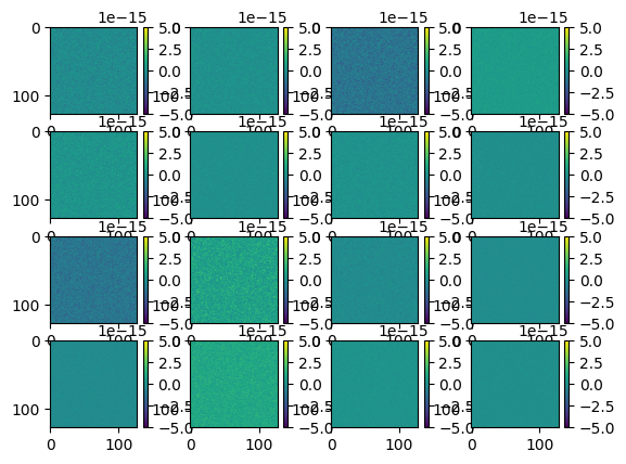
Please note that the scale of these plots is on the order of \(\pm 10^{-15}\), meaning that we’ve recovered the Mueller matrix to femto-scale precision, which is essentially our machine precision.

print('Machine Epsilon = ',np.finfo(float).eps)

Machine Epsilon =  2.220446049250313e-16

Of course, this precision means nothing in the presence of real noise sources so all we’ve learned is that katsu introduces a totally vectorized approach to Mueller polarimetry with absolutely no compromises to accuracy. In the next tutorial we will show how this can be applied in a laboratory setting.